Neglect of variation, analysis of variance, Part 2

My last article discussed the failure to consider variation in an experiment. I had no part in the project running that experiment. I will now discuss an experiment I conducted where I neglected to consider variation.

The experiment was to test the susceptibility of optical fibers to gamma radiation. I measured the attenuation (loss of optical transmittance) of the optical fibers as a function of radiation dose.

I ordered a spool of sample fiber from each manufacturer. I unspooled 20 meters of fiber. Snip, one specimen. I unspooled another 20 meters of fiber. Snip, a second specimen. I was now covered. Two specimens of each fiber. The data from the experiment at a given radiation dose looked like the sketch below.

But had I really allowed for variation? In retrospect, no. The two specimens were from the same spool. They were not independent samples. They would have identical raw materials and identical processing. From memory I recall that one of the parameters affecting radiation life of optical fibers is the hydroxyl concentration. But the two fibers from a specific manufacturer being of the same lot would have no variation in hydroxyl concentration.

They should have been from different production lots separated in time. This would allow for variation in the lots of raw materials and variation in process parameters. Because my samples were not independent I could not really say conclusively whether the data from multiple lots would look like this:

Or perhaps this:

In the second case there is no statistically difference between the fibers.

It is not enough to have multiple specimens. You must also understand the reason for having multiple specimens. The point of multiple specimens is to try to capture and understand the true variability in what you are studying.

tags:

Mechanical Engineering
Analysis of variance
ANOVA

Ignore this post

This post is for linking to technorati

Technorati Profile

Neglect of variation, analysis of variance

A common mistake in conducting experiments is to neglect variation. Engineers are quite prone to this. We tend to think in deterministic formulas. This leads us to ignore the effects of variation in conducting experiments. To best explain this I will give an example.

Please note: I was not involved in this experiment. I am recounting the events of the experiment as well as I observed them from the outside. Some of the details have been simplified to ease reporting on them in my blog.

There was an experiment conducted at my employer about six years ago. The goal of the experiment was to select a material resistant to cavitation erosion. The material was to go into a piping system where it would be subjected to severe cavitation.

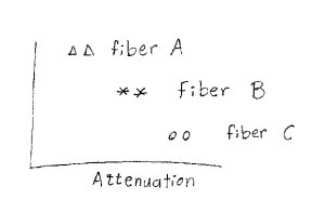
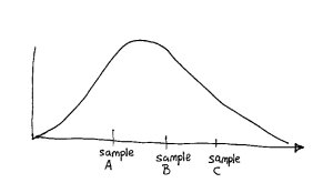
There was a sample tested for each candidate material. The testing entailed putting the sample under thermo-hydraulic conditions replicating those in the actual flow loop. After exposure to the test conditions the number of cavitation pits in the sample was counted. The data resembled something like that in graph below.

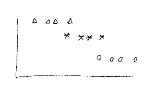
There were three materials tested. There was a count of cavitation pits per unit area for each material. The best material for the application is material A, right? What could be simpler than that?

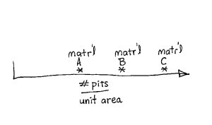
In selecting material A there is actually a hidden unstated assumption. The assumption is that there is little to no variation in the material properties. If you were to rerun the test with additional samples you would get essentially the same result. To word it another way there is a low coefficient of variation. . If this assumption is true and we run the test multiple times and we then plot the data from these tests as a probability distribution we would have something that would look like what is shown below, the data from the original actual test is indicated with the asterisk.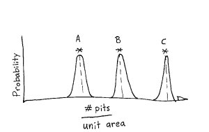

But the sad, ugly reality is that we cannot make that assumption without additional information. Material testing can have wide scatter in the data. Samples of nominally identical material but from different lots can have widely varying properties.

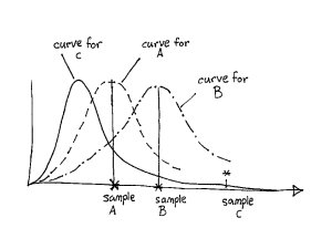
For all we know the probability distribution from running multiple samples would look like this:

Once again the actual data from the original test is shown with an asterisk. In this case there is no longer a significant difference in the behavior of the three materials. I am assuming that our one datapoint for each material falls at the mean. But based on the experimental data we can’t even be sure of that.

For all we know the distributions look like this:

In this case there is no difference in the three materials. All we have is three datapoints from a single distribution curve.

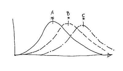
Worse yet, perhaps the true, unknown, distributions look like what is shown below here.

The one datapoint for C which did worse than our one datapoint for A and one datapoint for B is actually drawn from a distribution whose mean is better than that of A and B.

Based on the limited amount of data and no information as to what the distributions are there is no reliable way to select between materials A, B, or C.

The way to conduct a test such as this and make a reliable determination is to run multiples of each sample so we can distinguish the variation within a sample material and between sample materials. The statistical procedure to use is called analysis of variance or ANOVA.

tags:
Mechanical Engineering
Analysis of variance
ANOVA